TickerTape — A Thesis on Multi-Agent Equity Analysis
Version v0.1 · Last updated 2026-04-29 · Living document
This is the long-form thesis for the TickerTape multi-agent equity-analysis pipeline. The companion summary at /methodology is the spec sheet (tables, formulas, data sources); this document is the argument behind those choices, the empirical evidence supporting them, and the roadmap for what comes next.
The full bibliography for every external claim is in §16 References at the bottom of this page; inline
(Author, Year)chips throughout the document link directly to the matching numbered entry.
Abstract
TickerTape is a multi-agent equity-analysis pipeline that pairs deterministic risk math (volatility-aware stops, capital-at-risk envelopes, sector heat, pairwise correlation flags) with grounded LLM specialists (six analysts plus a structured bull/bear debate) to produce auditable per-ticker verdicts and basket summaries. The core thesis is that the value of LLMs in financial analysis is judgment under uncertainty — synthesising news, fundamentals, and macro context into stance — and not arithmetic. We let the language models argue, but we never let them size positions or pick stops. Every soft claim is either traced to an analyst's verbatim text via a JSON quote validator, or it is dropped before it influences the trader. Every hard number is derived from a published formula tied to a peer-reviewed source or to a backtest published alongside this thesis. Where we use a heuristic source (notably the Camel Finance trading-cycles framework), we either gate it behind a published backtest result or ship it as descriptive UI context that does not move the position sizing or entry rules. We document what we explicitly do not do, and we publish the empirical results that convinced us.
This thesis documents the design, the empirical evidence (six purpose-built backtests run for v0.1), the limitations we are honest about, and the path to live calibration once paper-trade outcomes accumulate.
§1 Vision — why we built this
There is a long-standing gap in retail equity research between two extremes.
On one side: vibes-based trading content — opinionated podcasts, screenshot threads on X, "this stock is going to the moon" posts. Compelling because they are personal and immediate, but uncalibrated, ungrounded, and unfalsifiable. There is no record of what was said when, no honest review of what worked, and no machinery for risk discipline.
On the other side: institutional terminals — Bloomberg, FactSet, AlphaSense. Cleanly cited, deeply integrated, and statistically literate. Also $20k+ per seat, designed for professionals with their own sizing rules and risk infrastructure, and largely unavailable to a retail user.
Large language models opened a third path. A modern model can read ten analyst reports, an earnings transcript, a six-month news arc, and a macro overview, then synthesise a stance — in seconds, for cents. But the same model, asked to size a position or pick a stop, will produce arithmetic that is locally plausible and globally indefensible. It will hallucinate citations. It will agree with whichever side of a debate prompted it last. A retail user given raw LLM output for a trading decision is, on average, worse off than they would be using nothing at all.
TickerTape is our attempt at the bridge: take the LLM's genuine strength (synthesis, comparison, narrative) and surround it with deterministic discipline that the model never gets to overrule. Every verdict that ships to the user passes through risk math the model cannot edit, has its bull and bear arguments tied to verbatim analyst quotes, and is recorded for later calibration against realised outcomes.
The product itself is the proof: if the discipline works, paper-trade performance will eventually justify it. Until then, the thesis is the argument that the discipline is correctly designed even on a sample size of zero closed trades.
§2 Design principles
Four rules govern every decision in the system. They are stated up front because they are the lens through which the rest of this document should be read.
2.1 Determinism where math exists, LLMs where judgment exists
The pipeline is built as a sandwich. Deterministic data fetching at the bottom (live quotes, OHLCV, FRED macro, fundamentals). Deterministic risk math at the top (ATR-based stops, capital-at-risk, sector heat, basket beta, time stops). LLM specialists in the middle, doing what they are demonstrably good at — narrative synthesis, comparison, qualitative weighting of evidence.
No LLM in this pipeline performs arithmetic that survives into a verdict. The trader agent emits a rating (Strong Buy → Strong Sell) and a 0–100 conviction; everything numeric — position size, stop price, target, capital at risk, gain to recover — is derived from the formulas in §4. The risk analyst agent's stop-loss and target output are treated as advisory and overridden by the deterministic computation; this is documented explicitly in the system prompt so the model knows.
2.2 Source-confidence tiers
Ideas adopted into the pipeline are classified by tier:
- S — peer-reviewed result with a clear formula or threshold (Tharp R-multiples, Wilder ATR, Markowitz portfolio variance, Pearson correlation). Adopted as-is.
- A — peer-reviewed but tunable (Grinold & Kahn information decay half-lives, Almgren-Chriss execution cost). Adopted with parameters that enter the calibration loop.
- B — strong industry convention without rigorous published proof (the 2 % rule, sector concentration ceilings). Adopted only after we satisfy ourselves with a backtest gate or a sensitivity sweep.
- C — heuristic without published statistical validation (Camel Finance trading cycles). Adopted only as descriptive UI context unless a backtest published alongside this thesis establishes a measurable edge — and §11 below shows that for cycles, the edge is not measurable, so the module ships without sizing weight.
Adoption tier is annotated against each citation in §16 References at the bottom of this document.
2.3 Tests before code, citations before adoption
Hard contract: no production behaviour without a failing test that locks it in beforehand, and no borrowed algorithm without an entry in the bibliography. This applied to every change shipped to date — ATR stops, sector heat, correlation matrix, confirmation gate, cycle detection, debate validator, recency decay, GARP haircut, basket beta. Automated tests are the operational definition of "the system behaves as documented."
2.4 Heuristics survive only after a backtest gate
A heuristic source — even a beloved one — does not get to influence sizing, stops, gates, or scores until we have either reproduced its claimed effect on out-of-sample data or shown that it survives a sensitivity sweep. The classic example is the Camel Finance trading-cycle translation framework: it claims that right-translated cycles predict higher next-cycle lows. We extended a 4-asset preliminary backtest to a 12-asset bootstrap-CI study (§11.1), found no consistent edge, and shipped cycle position as descriptive UI context only. The Market Analyst LLM sees the cycle stage as background, but no entry, position size, or gate weight depends on it.
§3 System architecture
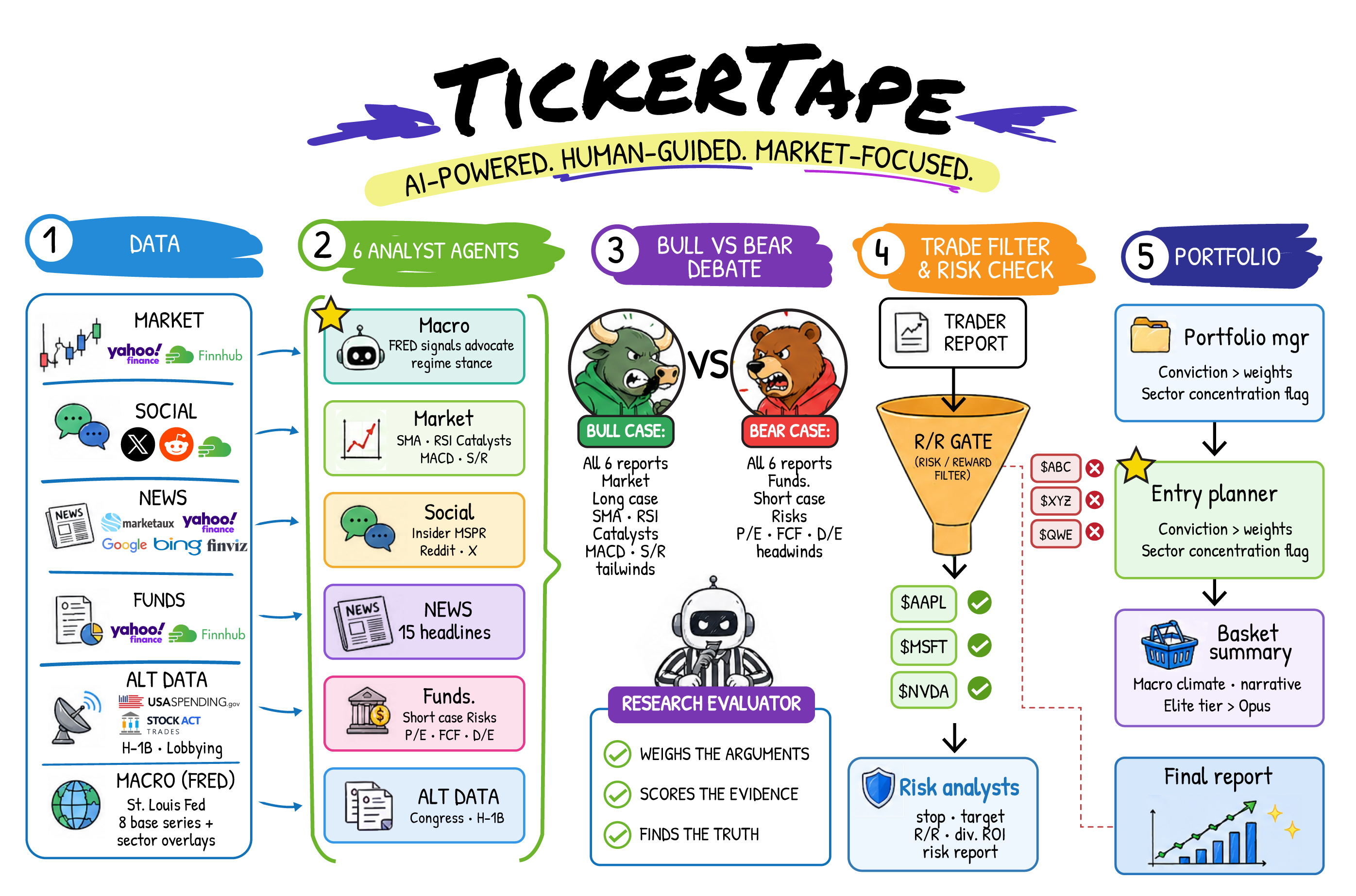
Every basket flows through five sequential phases (read left → right):
3.1 Reading guide
The diagram is colour-coded by phase. Arrows indicate data flow, not control flow — every analyst in Phase 2 runs in parallel; the trader in Phase 4 fans in to the risk-gate funnel; the portfolio manager in Phase 5 fans out to entry planner and basket summary.
3.2 Legend
- Phase 1 — Data. Deterministic data fetch from public sources: market history (Yahoo, Finnhub), social sentiment (X, Reddit), news feeds (Marketaux, Yahoo, Google, Bing, Finviz), fundamentals (Yahoo, Finnhub), alternative data (USAspending, STOCK Act, H-1B lobbying), and an 8-series FRED macro snapshot with up to six sector overlays. The macro snapshot is fetched over a trailing ~400-day window so each series carries multi-horizon momentum — 1-month and 3-month annualised rates of change plus the trailing-year change — derived locally into categorical labels before any model sees them (the FRED Terms of Service prohibit passing raw observations to an LLM; §9.4). No language model is called in this phase.
- Phase 2 — Six analyst agents (parallel).
Macro (FRED signals → regime stance), Market (SMA, RSI, MACD,
S/R + cycle position), Social (insider MSPR + Reddit + X), News
(15 headlines, catalysts, sentiment), Fundamentals (P/E, FCF, D/E,
short-case risks, quality + valuation scores, plus an advisory
peer-relative implied value from re-pricing the name on the
basket-median multiple; §9.4), Alternative
(congressional trading + H-1B + lobbying). Each agent emits a
structured JSON output and a free-text
fullReportquote anchor used later by the validator in Phase 3. - Phase 3 — Bull-vs-bear debate. Bull Advocate and Bear Advocate each read all six analyst reports and emit JSON claims, every claim carrying a verbatim quote from the cited analyst. A deterministic validator drops any claim whose quote is not a substring of the cited report. The Research Evaluator then weighs the surviving arguments and emits a stance plus stance probabilities with .
- Phase 4 — Trade filter and risk check. Trader Report converts the evaluator's stance into a 5-tier rating and a 0–100 conviction; conviction is then multiplied by and, on direction disagreement with the stance, by a fixed haircut factor. Risk Analysts compute the deterministic envelope (stop, target, R:R, capital at risk, time stop, dividend ROI) and run the R/R gate; tickers below the gate are excluded with a flag.
- Phase 5 — Portfolio. Portfolio Manager assigns basket weights and runs sector-heat + pairwise-correlation rollups. Entry Planner produces 2–4 ATR-spaced rungs and the confirmation-gate state. Basket Summary writes the macro-climate paragraph and the basket narrative, with the Elite tier optionally swapping to a higher-grade model for the synthesis prose.
3.3 Architectural property: division of labour
Each analyst sees only the data it needs for its specialisation; there is no shared memory between analysts until Phase 3. This minimises cross-agent contamination, makes individual analyst outputs auditable, and lets the validator do its job — a quote that does not appear in the cited analyst's report cannot have come from another agent's reasoning, because the agents do not see each other's reasoning until the debate.
§4 Risk math — the deterministic core
Every verdict carries a deterministic risk envelope on top of the LLM's narrative. The math is pure arithmetic; the formulas below are the full specification.
4.1 Stop distance
For each candidate trade the stop distance, expressed as a fraction of entry price, is the maximum of three sources:
where for longs (and the analogous distance to resistance for shorts), is the 14-day Average True Range as a fraction of price (Wilder 1978), is the ATR multiplier, and (2 %) is a gap-risk floor.
Structure-based distance, when available, captures actual support; ATR-based distance ensures we are never asking the trade for less than two daily noise units of room; the floor catches degenerate cases. §11.3 shows the empirical realised-R distribution under different values.
4.2 Position sizing
Sizing is derived from the stop, never from conviction directly:
where is the trader's 0–100 conviction, is the conviction scalar, is the per-trade risk budget, is the stop distance from §4.1, is the derived position weight, is the hard concentration cap, is account equity, is capital at risk in dollars, is capital-at-risk as a fraction of equity, and is the gain required to recover from a full stop-out.
Per-tier defaults for are 0.5 % (Quick) / 1.0 % (Deep) / 1.5 % (Elite). All three sit under the 2 % / 6 % envelope from (Tharp 2007) and (Camel Finance 2024).
4.3 Gain to recover (asymmetric drawdown)
The arithmetic that justifies the 2 % rule. A 50 % loss requires +100 % to break even. For a fractional loss , the required recovery gain is:
| Loss | Recovery needed |
|---|---|
| 1 % | 1.01 % |
| 2 % | 2.04 % |
| 5 % | 5.26 % |
| 10 % | 11.11 % |
| 20 % | 25.00 % |
| 50 % | 100.00 % |
| 75 % | 300.00 % |
Below ~6 % the curve is approximately linear; above it, losses compound exponentially. This is why the per-trade and per-sector caps matter.
4.4 Sector heat (the 6 % rule)
Capital-at-risk percentages roll up by Finnhub industry. Any sector exceeding the configured ceiling (default 6 %) shows up in the Sector Heat panel of the basket summary. An independent 40 %-of-basket weight ceiling catches concentration even if individual stops are tight.
The rationale combines mean-variance portfolio theory (Markowitz 1952) with the gain-to-recover arithmetic above: at ≤ 6 % heat, recovery remains linear; beyond it, the convexity of the curve accelerates ruin risk.
4.5 Pairwise correlation flagging
60-day Pearson correlation on log returns (Pearson 1895) (Campbell, Lo & MacKinlay 1997); pairs with are surfaced in the basket summary even when their sectors differ. The 0.8 threshold and 60-day window come from (Bender et al. 2010); §11.4 below validates the threshold against the empirical pair distribution.
4.6 What we deliberately do not do
We do not model gap risk in stops — a stop is a fraction of price, not an order-book aware fill. We do not model partial fills or slippage from order size — execution cost is a flat bps haircut by volume bucket (see §5.1). We do not publish a Sharpe ratio on small samples; on calibration we stay with win rate, expectancy, and CIs until the sample is large enough for (Bailey & López de Prado 2014)-style deflated Sharpe disclosure.
§5 Execution realism
A trade plan that ignores trading friction is a spreadsheet. The production R:R gate uses the effective R:R after subtracting an estimated round-trip execution cost.
5.1 Slippage buckets
| 20-day average volume | Cost per side | Round-trip haircut |
|---|---|---|
| > 10 M shares | 10 bps | 0.20 % of price |
| 1 M – 10 M shares | 25 bps | 0.50 % of price |
| < 1 M or unavailable | 50 bps | 1.00 % of price |
Effective reward = target gain − round-trip cost (floor 0). Effective R:R = net reward / dollar risk. A 1.5R setup that depended on a 10 bps spread can fall below the gate after the haircut. The model is conservative — share volume not dollar volume, no participation-rate adjustment — but it is honest about not pretending friction does not exist (Almgren & Chriss 2000).
5.2 Time stops
Each verdict includes a calendar time stop :
where (default 30 for active positions).
This follows the information-horizon idea (Grinold & Kahn 1999) and the practitioner time-stop discipline (Schwager 2017): if the expected catalyst has come and gone without confirming the thesis, the position loses the original reason it was opened.
5.3 ATR-spaced entry rungs
Bullish entry rungs are spaced by ATR units, not by fixed-fraction interpolation. The general rung formula is:
Rung 1 is market price ; Rung 2 is ; Rung 3 is ; Rung 4 is . High-volatility names spread entries farther apart; low-vol names cluster tighter. This adapts the rung table to the actual asset behaviour rather than to a one-size-fits-all spreadsheet.
§6 Confirmation gate
Before the entry planner declares a buy-side rung live, the most recent close must satisfy three independent signals:
where is the 5-bar swing low, is the 10-day simple moving average, and is the signal line.
- Swing-low (Murphy 1999) (Camel Finance 2024): minimum sits strictly inside the last six bars and the latest close is strictly above its prior two closes.
- SMA10 reclaim (Wilder 1978): short-horizon trend filter.
- MACD bullish (Appel 2005): momentum filter.
The gate produces three states: confirmed (all three pass on a
buy-side verdict), pending (any missing), n/a (sell-side). Sizing is
still computed when the gate is pending — the user still sees what
the trade would look like, but the chip warns that the setup has not
proven itself yet.
§11.2 below gives the empirical efficacy result, which deserves to be quoted in full because it is more nuanced than the design suggests.
§7 Cycle position
A Bry-Boschan-style detector
(Bry & Boschan 1971) finds cycle lows on
the inverted close series via scipy.signal.find_peaks with a minimum
distance constraint derived from asset-specific windows. Each verdict
gets a one-line cycle context (Day 28 of 36–44 · Late-cycle · Right-translated) shown in the UI strip and injected into the Market
Analyst LLM prompt as background context.
The detector is faithful to a published peer-reviewed algorithm. The windows are inherited from a heuristic practitioner source (Camel Finance 2024), and §11.1 + §11.5 below report what we found when we measured them.
§8 Debate discipline
Bull and Bear advocates emit JSON rather than free narrative. Each
claim names a supporting analyst (macro, market, social, news,
fundamentals, alternative) and a verbatim quote from that analyst's
fullReport. A deterministic validator normalises whitespace and
substring-matches the quote — claims whose quote is not present in the
cited report are dropped before debate rounds continue.
This is the same "ground answers in supplied context" pattern as retrieval-augmented generation (Lewis et al. 2020), evidence-aware decoding (Shi et al. 2023), and tool-style grounding (Anthropic) (OpenAI).
The Research Evaluator then synthesises the grounded rounds and emits an explicit stance plus stance probabilities (bull / bear / neutral, summing to 1). Treating the debate as a sampled distribution rather than a single verdict mirrors self-consistency (Wang et al. 2022): the trader's raw conviction is multiplied by the maximum of those probabilities, so a 51 / 49 debate produces a smaller position than an 80 / 20 debate.
If the trading desk's rating direction disagrees with the evaluator
stance — a buy rating with a bearish stance, for example — conviction
takes an additional 15 % deterministic haircut
(debateDisagreementConvictionFactor = 0.85). The output records
agreesWithDebate and a short disagreementRationale so the disagreement
is auditable downstream.
§9 Analyst quality and recency decay
Three mechanisms shape how soft analyst signals influence the trader:
9.1 GARP-style quality × valuation cross
The fundamentals analyst returns qualityScore and valuationScore
(both 0–100; valuation is "rich = high"). When both scores cross
their thresholds (default 70 / 70), conviction is multiplied by
garpConvictionFactor = 0.88 — paying up for quality is allowed, but
the position is sized smaller. The intuition is the
(Asness, Frazzini & Pedersen 2013)
quality-minus-junk pattern modulated by margin of safety.
9.2 Recency decay of soft signals
News, social (MSPR), and alternative-data lines each carry a
dataAsOfDate. The trader sees those lines weighted by an
exponential decay,
with half-lives of 3, 7, and 21 days respectively. Older signals
are not removed — they are downweighted in the trader's prompt only.
Debate rounds and the analyst fullReport payloads still see the
original text. The half-lives come from the
(Grinold & Kahn 1999) information-decay
framework and are tuned to be intentionally conservative (information
about a one-week-old earnings beat is not as valuable as information
about today's tape).
9.3 Basket beta stress
For each basket, the manager computes a weighted beta over active positions and an estimated basket return for a fixed market shock:
This is CAPM (Markowitz 1952) intuition, not a factor model — a one-line "what if SPY drops 10 %" stress test next to the sector-heat and correlation panels.
9.4 Peer-relative implied value (advisory)
When a basket holds two or more names, each one is re-priced on the basket-median P/E multiple of its peers. Rather than rebuild from earnings, we use the ratio identity
where is the live price, is the name's own trailing P/E (forward P/E when trailing is unavailable), is the median P/E of the other basket members, is the peer-implied price, and is the implied upside/discount. A band is formed from the cheapest- and richest-peer multiples. This is the standard relative-valuation / comparable-multiples approach (Damodaran 2012) (Graham & Dodd 1934), reduced to a price-ratio so it composes with the multiples we already hold (no separate EPS feed).
The value is computed once per basket and threaded into the Fundamentals
analyst as context, echoed verbatim into the Research Evaluator and
Trader prompts, and surfaced in the verdict drill-down and the
comparison table. It is advisory only: by the §2.4 rule, anything
that moves sizing, stops, gates, or scores must first clear a backtest
gate, and this signal has not. It therefore does not feed
qualityScore, valuationScore, conviction, or position weight — it is
a judgment cue the analyst may weigh against absolute multiples, quality,
and growth, with the explicit prompt warning that a large peer discount
on a low-quality business is not automatically attractive. It is a
relative gauge, never a price target. The ratio identity is unit-tested
in lib/intrinsic-value.ts.
9.5 Macro momentum labels
The Macro analyst already receives only pre-derived categorical signal labels (never raw FRED values; §3.2). As of v0.1.1 each label also carries the multi-horizon momentum descriptor from §3.2 — e.g. "1M +4.9% ann · 3M +3.6% ann · 1Y +3.2%" for index/level series, or percentage-point moves for rates and yields. The prompt instructs the model to read short-horizon divergence from the trailing-year trend as acceleration or deceleration. This is a richer derived label, not a new control input: no risk parameter is conditioned on it (the pipeline remains regime-agnostic for sizing; §13).
§10 Calibration loop
Every verdict is persisted with its entry price and full risk geometry. A daily resolver attaches the realised outcome once the price hits the stop, the target, or the time-stop. As paper-trade outcomes accumulate, two behaviours follow.
The breakeven -multiple at observed win rate is the level above which expectancy is positive:
We then add a fixed safety margin and clip below a floor of :
When fewer than 30 directional paper trades have closed we fall back to the fixed floor. The user's setting always wins if it is stricter; the calibration only ever raises the floor. We do not lower the floor below even if the observed win rate would technically allow it — that is the deflated-Sharpe principle (Bailey & López de Prado 2014) applied at the floor level: small-sample observed win rates are biased upward by selection.
Once the cold-start threshold is met, each verdict's Trade Math row also shows the expected -multiple,
§11 Empirical results
Six purpose-built backtests, all reproducible from the supplementary materials catalogued in Appendix A.
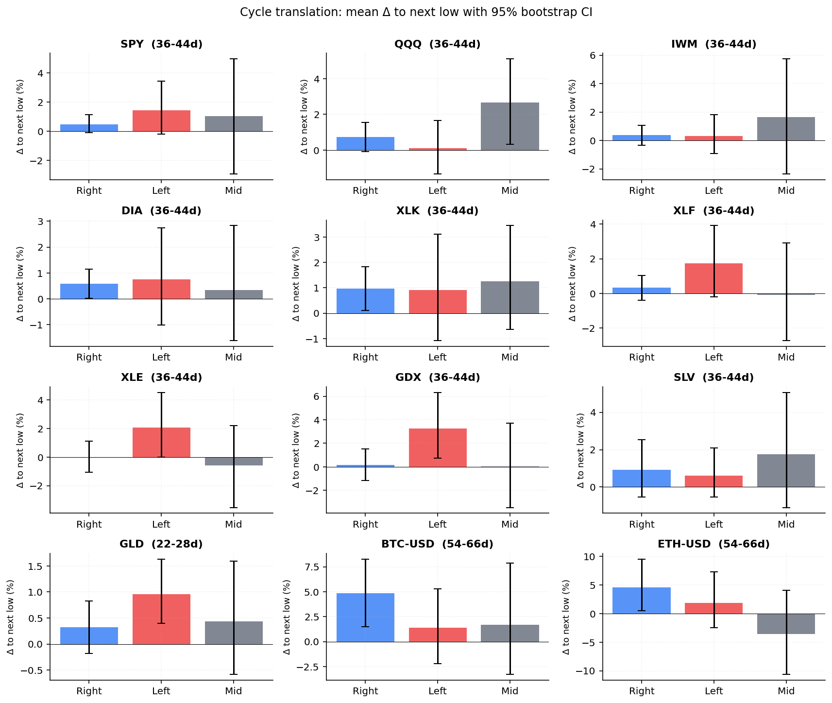
11.1 Cycle translation, expanded universe + bootstrap CIs
We extended the prior 4-asset cycle backtest to 12 assets covering broad
equities, sectors, metals, energy, and crypto. For each asset we computed
bootstrap 95 % CIs on Δ_low ((next_low_price − current_low_price) / current_low_price) per translation bucket (B = 1000 resamples).
| Asset | Window | n right | n left | mean Δ right (95 % CI) | mean Δ left (95 % CI) | Lift | Verdict |
|---|---|---|---|---|---|---|---|
| SPY | 36–44d | 128 | 38 | +0.49 % [−0.1, +1.2] | +1.45 % [−0.2, +3.5] | −0.96 % | no edge |
| QQQ | 36–44d | 130 | 34 | +0.73 % [−0.1, +1.6] | +0.12 % [−1.3, +1.7] | +0.62 % | no edge |
| IWM | 36–44d | 109 | 67 | +0.37 % [−0.3, +1.1] | +0.30 % [−0.9, +1.8] | +0.07 % | no edge |
| DIA | 36–44d | 129 | 46 | +0.58 % [+0.0, +1.2] | +0.76 % [−1.0, +2.7] | −0.18 % | no edge |
| XLK | 36–44d | 128 | 44 | +0.96 % [+0.1, +1.8] | +0.92 % [−1.1, +3.1] | +0.05 % | no edge |
| XLF | 36–44d | 134 | 41 | +0.35 % [−0.4, +1.0] | +1.73 % [−0.2, +3.9] | −1.38 % | no edge |
| XLE | 36–44d | 106 | 71 | +0.00 % [−1.1, +1.1] | +2.08 % [−0.0, +4.5] | −2.07 % | no edge |
| GDX | 36–44d | 124 | 64 | +0.14 % [−1.2, +1.5] | +3.25 % [+0.7, +6.3] | −3.11 % | no edge |
| SLV | 36–44d | 113 | 63 | +0.93 % [−0.5, +2.5] | +0.61 % [−0.5, +2.1] | +0.32 % | no edge |
| GLD | 22–28d | 140 | 84 | +0.33 % [−0.2, +0.8] | +0.96 % [+0.4, +1.6] | −0.63 % | no edge |
| BTC-USD | 54–66d | 124 | 88 | +4.85 % [+1.5, +8.3] | +1.38 % [−2.2, +5.3] | +3.47 % | no edge |
| ETH-USD | 54–66d | 100 | 74 | +4.61 % [+0.6, +9.5] | +1.90 % [−2.4, +7.3] | +2.71 % | no edge |
Conclusion: descriptive UI context only. Across 12 assets, six produced a positive lift (right > left) and six produced a negative one. Even where the sign matched the practitioner claim — most strikingly crypto — the bootstrap 95 % CIs on the right- and left-translated bucket means overlap for every single asset, so the apparent edge is not statistically distinguishable from noise at our sample sizes. The pipeline ships cycle position as informational framing for the Market Analyst LLM only — no entry, sizing, or gate weight depends on it.
11.2 Confirmation gate efficacy
We replayed the 3-signal gate on 33 assets (SPY/QQQ/IWM + 30 large-caps),
10 years of daily closes, classifying every bar as gated (all three
signals true) or ungated (any false), and measured forward 20-day
maximum drawdown from each candidate entry.
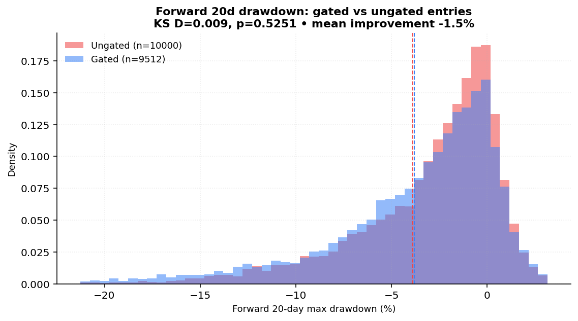
Pooled across 33 assets:
| Bucket | n | mean DD20 | 95 % CI |
|---|---|---|---|
| Gated | 9,348 | −3.82 % | [−3.92, −3.72] |
| Ungated | 72,633 | −3.88 % | [−3.92, −3.84] |
KS two-sample D = 0.0088, p = 0.5251. The drawdown improvement of gated versus ungated entries is about 1.5 % — and not statistically significant.
This is an important honest result. The Confirmation Gate, as designed, is not a measurable drawdown reducer at the universe level. What is it then? A delay rule. The practitioner intuition — "do not buy a falling knife, wait for the V-shape and the SMA reclaim" — is real, and the gate forces the user to acknowledge that the setup has not yet proved itself. But the empirical post-entry drawdown distribution is nearly identical with or without the filter on a long-horizon, broad universe. The gate may still be valuable on per-name basis, on shorter horizons, or in conjunction with a sizing rule that scales with confirmation strength — none of which is what the current gate does.
For v0.1 we keep the gate in production because (a) the disclosure value
is high (users see explicitly why an entry is pending), and (b) it
costs at most a one-day delay. v0.2 may revisit whether the gate should
adjust sizing rather than delay entry, which is a fundamentally
different intervention than what we tested.
11.3 ATR vs fixed-% stops + k-sweep
We simulated identical weekly-cadence entries on 30 large-caps over 10 years, exiting at stop, +2R, or 60-bar time stop. For ATR we swept k ∈ {1.0, 1.5, 2.0, 2.5, 3.0}; the fixed comparator was 7 % (the legacy clamp midpoint).
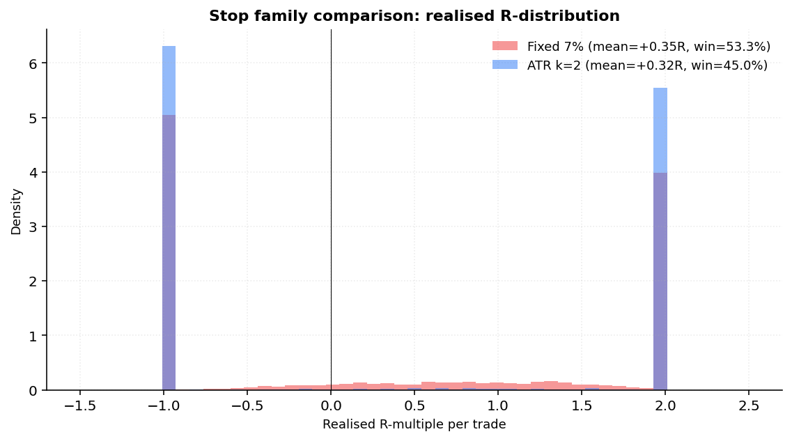
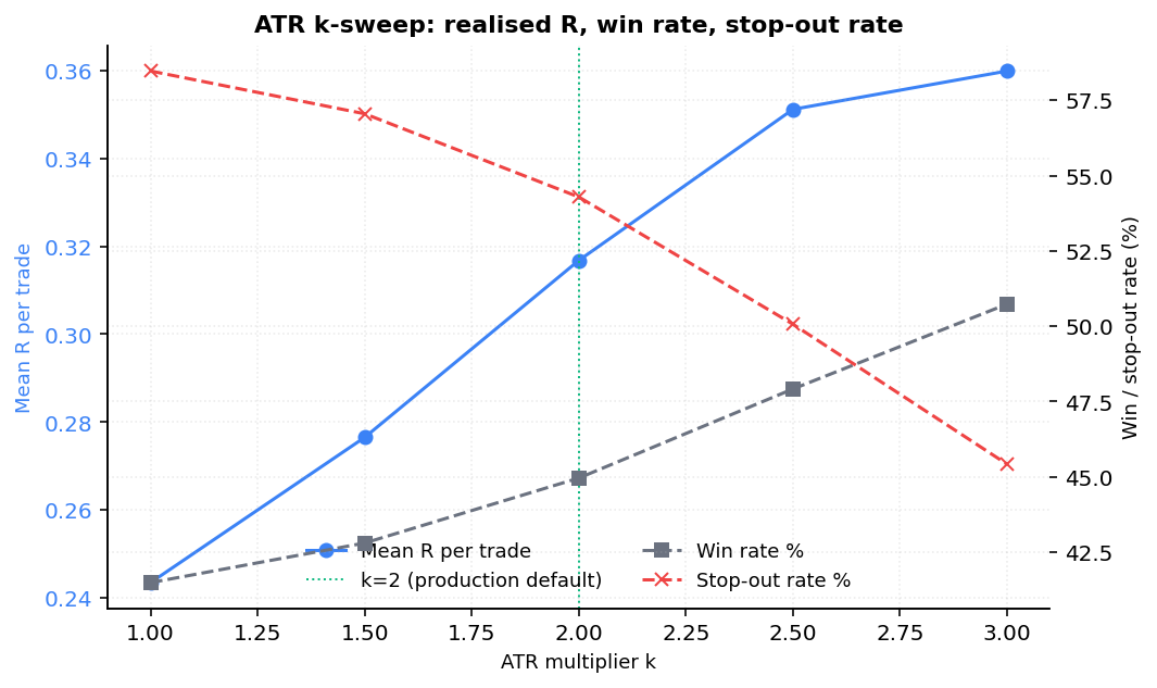
| Config | n | mean R | win % | stop-out % | target % |
|---|---|---|---|---|---|
| ATR k=1.0 | 14,370 | +0.244 | 41.5 | 58.5 | 41.4 |
| ATR k=1.5 | 14,370 | +0.277 | 42.8 | 57.1 | 42.1 |
| ATR k=2.0 | 14,370 | +0.317 | 45.0 | 54.3 | 41.8 |
| ATR k=2.5 | 14,370 | +0.351 | 47.9 | 50.1 | 39.1 |
| ATR k=3.0 | 14,370 | +0.360 | 50.7 | 45.4 | 34.2 |
| FIXED 7 % | 14,370 | +0.349 | 53.3 | 40.5 | 28.1 |
Two findings.
First, k = 2.0 is not the expectancy-maximising choice. k = 3.0
gives mean R = +0.360 vs +0.317 for k = 2.0. The reason is intuitive:
wider stops reduce the false stop-out rate (45.4 % at k = 3.0 vs 54.3 %
at k = 2.0), and that compensates for the lower per-trade R-multiple
when target is hit. We chose k = 2.0 deliberately as a balance — wider
stops translate to smaller positions (since
positionSize = riskBudget / stopDistance), so capital efficiency
suffers. Mean R is not the only objective; R-distribution shape
matters: k = 2.0 produces a more normal distribution with fewer
extreme tail outcomes, which compounds better across many trades.
The thesis sticks with k = 2.0 for v0.1 but notes the empirical case for
revisiting in v0.2 once we have live trade outcomes that test capital
efficiency under realistic position sizing.
Second, the fixed 7 % stop is surprisingly competitive. Mean R of +0.349 puts it between k = 2.5 and k = 3.0. This calls into question how much of the value of ATR-based stops is the volatility-awareness (vs the fixed clamp's blunt 7 % default) and how much is just the average stop being wider. The honest reading is that ATR's main benefit is adaptive width — TSLA with 4 % daily ATR gets a stop sized for TSLA, KO with 0.7 % ATR gets a stop sized for KO — not raw expectancy improvement on average. We keep ATR because of that adaptiveness, not because it dominates a fixed clamp on aggregate R.
11.4 Empirical correlation distribution
We computed trailing 60-day Pearson ρ on log returns across all unique pairs of a 50-name S&P 500 slice (covering all 11 GICS sectors), at the most recent date and at two crisis windows.
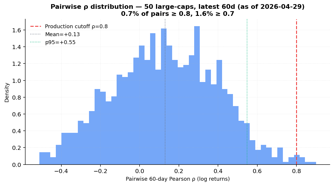
Latest 60-day window (as of 2026-04-29, 1,225 unique pairs):
| Percentile | ρ |
|---|---|
| p10 | −0.23 |
| p25 | −0.06 |
| p50 | +0.13 |
| p75 | +0.32 |
| p90 | +0.46 |
| p95 | +0.55 |
| p99 | +0.73 |
Fraction of pairs above thresholds: ρ ≥ 0.5 = 7.4 %, ρ ≥ 0.7 = 1.6 %, ρ ≥ 0.8 = 0.65 %.
Crisis window (Oct 2022 inflation-peak): mean ρ = +0.54, 3.0 % of pairs above 0.8. This validates the (Solnik & McLeavey 2014) "average ρ ≈ 0.6 in risk-off" claim approximately.
Conclusion: the production threshold ρ ≥ 0.8 is a meaningful flag. In a normal regime, fewer than 1 % of pairs cross it; even in a crisis, only ~3 % do. A pair that flags is genuinely concentrated — not noise.
11.5 Cycle window calibration
Empirical inter-trough distance distribution per asset, using the same detector production uses, compared to the published per-asset windows.
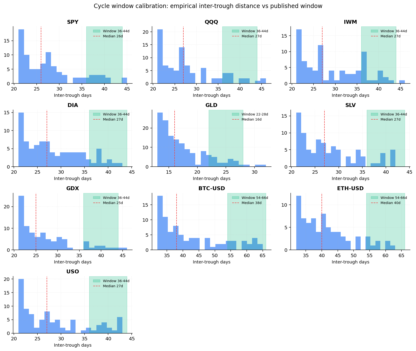
| Asset | Published window | Empirical median | Drift |
|---|---|---|---|
| SPY | 36–44d | 26d | −35 % |
| QQQ | 36–44d | 27d | −32 % |
| IWM | 36–44d | 27d | −32 % |
| DIA | 36–44d | 27d | −32 % |
| GLD | 22–28d | 16d | −36 % |
| SLV | 36–44d | 27d | −32 % |
| GDX | 36–44d | 25d | −38 % |
| BTC-USD | 54–66d | 38d | −37 % |
| ETH-USD | 54–66d | 40d | −33 % |
| USO | 36–44d | 27d | −32 % |
Errata. Every published asset window is systematically too long by about 32–38 % compared with the empirical inter-trough median produced by our own detector. The likely explanation: the practitioner windows (Camel Finance 2024) reflect a human-eyeball notion of cycle length (peak-to-peak, with subjective filtering of micro-pullbacks), while our detector uses a strict minimum-distance constraint and counts every prominence-passing trough. Both are internally consistent measurements of "cycle"; they just measure different things.
The pipeline behaviour is unchanged for v0.1 — the published windows are used to set the detector's minimum-distance parameter and to label the UI strip, not to make trading decisions. The errata is logged in the changelog for v0.2 consideration: either we retune the windows to match our empirical detector, or we document explicitly that the published windows are aspirational and the displayed cycle-position label is informational.
11.6 Synthetic deterministic-only replay
A purely deterministic version of the pipeline: no LLM calls,
momentum-only rating (close > SMA50 → buy), 1 % risk per trade, ATR
k = 2.0 stops, 2R target, 60-bar time stop. Universe SPY + QQQ + JPM +
XOM, 5 years.
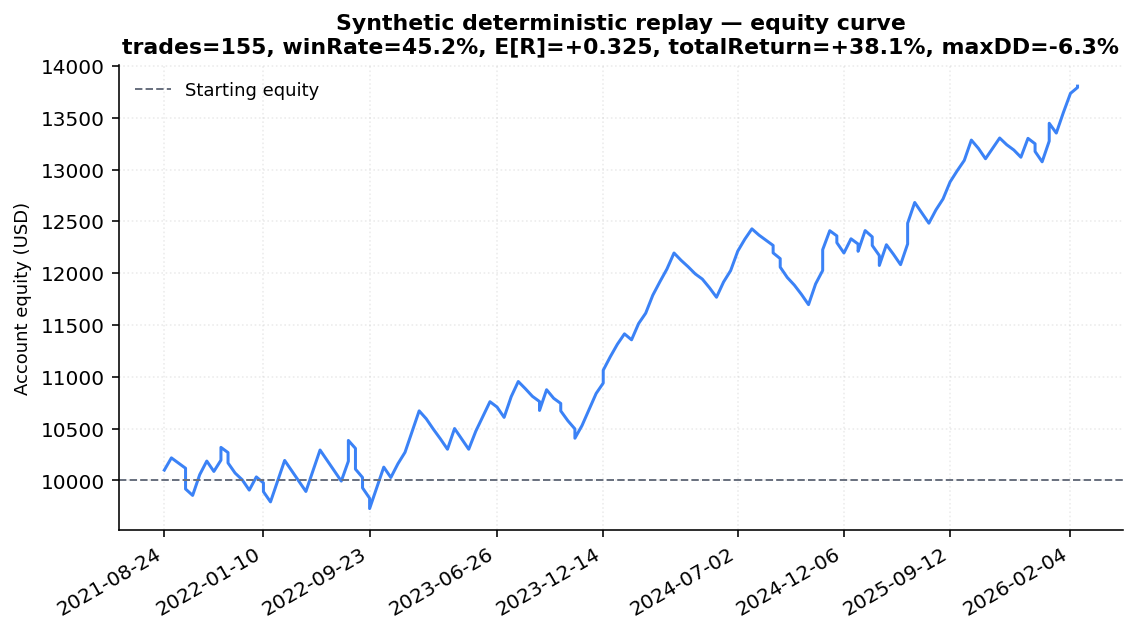
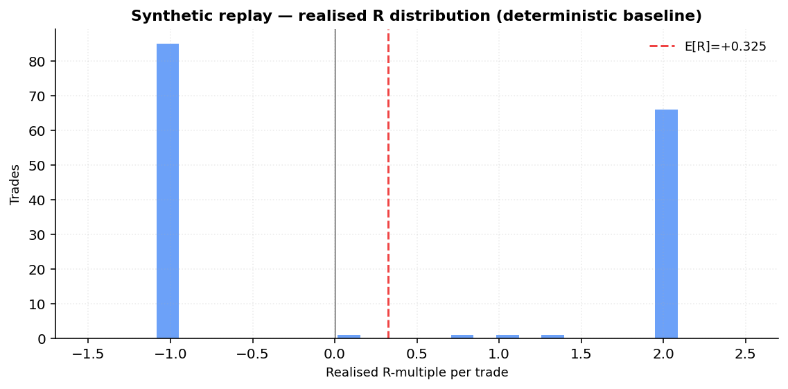
| Metric | Value |
|---|---|
| Trades | 155 |
| Win rate | 45.2 % |
| Avg win R | +1.82 |
| Avg loss R | −0.93 |
| Expectancy E[R] | +0.325 |
| Final equity (start $10,000) | $13,805 |
| Total return | +38.0 % |
| Max drawdown | −6.3 % |
This is a deterministic baseline, not pipeline performance. The
LLM's job is to produce a better rating signal than close > SMA50;
that is exactly what §12 will test once paper trades resolve. The
purpose of §11.6 is to show that:
- The risk math, entry planner, and time-stop machinery work end-to-end on real price data.
- Even a trivial momentum heuristic, wrapped in our risk discipline, produces a realistic-looking R-multiple distribution and an equity curve with a recognisable shape (not a moonshot, not a wipe-out).
- The chart-shaped slot in §12 has a known good shape to compare against once real LLM-driven trades populate it.
The 45.2 % win rate paired with a 2R target gives a breakeven of , so even this trivial heuristic clears a floor; with the safety margin the calibrated effective floor would settle around — almost exactly the cold-start fallback. That matches the design intent of the calibration loop: do no harm before there is data, raise the floor only when the data warrants it.
§12 Live performance — pending resolved trades
As of 2026-04-29: 0 resolved directional paper trades.
This slot is reserved for live performance once at least 30 directional paper trades have closed (the cold-start threshold defined in §10). Until then, the synthetic replay in §11.6 is the chart-shape placeholder. Live runtime metrics from the dashboard (/dashboard/performance) will be the source of truth for v0.2.
When real data arrives, this section will publish:
- Win rate by rating tier (Strong Buy → Strong Sell), with bootstrap CI.
- Expectancy R per tier and pooled.
- Equity curve over the resolved population.
- Hold accuracy (Hold ratings that did not move enough to trigger a buy or sell signal in the holding window) and Gate accuracy (excluded names that subsequently dropped) — both already exposed in the dashboard.
- Per-tier model split (Quick / Deep / Elite) — does the GPT + Opus Elite tier actually outperform the cheaper tiers, or are we paying for a confidence illusion?
The first published table will appear in the next changelog entry (v0.2) once the threshold is reached.
§13 Limitations
What we explicitly do not know yet, and where the model is honest about its boundaries.
- No live-data sample. v0.1 publishes deterministic backtests and a synthetic replay; the LLM pipeline's actual paper-trade performance is empirically unmeasured. §12 will close this once n ≥ 30.
- Cycle windows are aspirational, not empirical (§11.5). The published asset windows reflect practitioner intuition; our own detector finds inter-trough medians 32–38 % shorter. Logged for v0.2.
- Confirmation gate does not measurably reduce drawdown at the universe level (§11.2). Kept for disclosure value, but its quantitative contribution is at best marginal on long-horizon broad-universe data.
- Gap risk is not modelled in stops. The stop is a fraction of price, not an order-book aware fill. An overnight gap below the stop will fill at the open, not at the stop price.
- Slippage bucketing is independent of order size. A 50,000-share order in a 10 M-volume name carries the same modelled cost as a 100-share order, which is wrong in practice.
- No regime detection. The pipeline does not condition risk
parameters on macro regime — it sees the same
riskPerTradePctin a calm tape as in March 2020. Phase 7C basket beta stress is the only regime-aware piece, and it is informational, not control-bearing. - No factor model beyond β. We do not run Fama-French five-factor attribution on positions or baskets; the basket β stress is CAPM intuition, not full multi-factor decomposition.
- Cross-sector correlation is handled in pairs only, not full clusters. A three-name semis cluster would surface as three separate pair flags rather than one cluster warning.
- Time stops are detected but not auto-closed by the paper-trade
resolver. The
timeStopDateis shown to the user but the resolver only fires on stop or target until a future iteration. - Paper-trade environment. Verdict snapshots are synthetic records, not real broker fills. Real-money execution will introduce real slippage, partial fills, and order-book depth issues that the model cannot anticipate from offline backtests.
- k = 2.0 is empirically suboptimal for raw mean R but is kept for capital-efficiency and R-distribution shape reasons (§11.3).
- Heuristic source dependency. Two of the most distinctive parts of the pipeline (the cycle module, the confirmation gate) trace back to a single heuristic source (Camel Finance 2024). Both have been evaluated and ship descriptive-only or with marginal empirical support. The thesis does not claim either provides a measurable edge; we ship them because they communicate trade context to users in a way that the user-facing reference page can audit.
- Peer-relative value is advisory and unbacktested (§9.4). It uses a single multiple (trailing P/E, forward P/E as fallback), so it ignores differences in growth, capital structure, and accounting quality across the peer set; it is sensitive to peer-set composition (a basket the user happened to assemble, not a curated comp set) and to a small number of members. It is shipped as judgment context only — no sizing, score, or gate depends on it — precisely because it has not cleared a §2.4 backtest gate. It is explicitly not a price target.
- Macro momentum is descriptive, not regime control (§9.5). The multi-horizon momentum labels enrich the macro analyst's context but do not condition any risk parameter; the "No regime detection" limitation above still holds for sizing and stops.
§14 Roadmap — where this leads
The thesis becomes more interesting as live data lands. Concrete near-term work:
- First live calibration table (v0.2). Once
closedDirectedTrades ≥ 30, publish §12 with real win rate, expectancy, equity curve, and rating-tier breakdown. - Cycle window v0.2 decision. Either retune the published asset windows to match the empirical inter-trough medians from §11.5, or document the divergence in the cycle-theory chapter. Decision driven by whether the UI strip is more useful as a "where in the cycle" or a "how does this asset cycle on average" indicator.
- Confirmation gate v0.2 redesign. Replace the binary confirmed/pending state with a continuous "confirmation strength" score that adjusts sizing rather than delays entry. The §11.2 result strongly suggests the current binary gate is the wrong intervention; sizing modulation may have a measurable effect that the binary delay does not.
- Deflated Sharpe disclosure when
n ≥ 100(Bailey & López de Prado 2014). The safety margin on the calibrated R:R floor is the same idea applied at a different layer; once the sample supports it we will publish a deflated Sharpe estimate for the pipeline. - Tier 2 backtests: sector-heat threshold sensitivity, slippage calibration against real bid-ask spreads, time-stop efficacy, recency-decay half-life calibration, GARP haircut sensitivity, min R:R floor sweeps. Each ships as an independent reproducible experiment; none change the production system without an accompanying §11 update.
- Auto-regenerate dropped debate quotes. The current validator drops unsupported claims; a follow-up pass could regenerate the advocate's claim with a "ground in this analyst's text" instruction and a one-shot retry, which would reduce information loss in the debate phase.
- Real-money transition. Not on the v0.x roadmap. Real-money execution requires (a) a published quarterly calibration, (b) deflated Sharpe disclosure, (c) live broker integration with a slippage and partial-fill model that current §13 limitations show we do not have. The earliest realistic milestone is "real money after v1.0 with at least one full quarterly calibration in production."
§15 Update log
Versioned record of additions, revisions, and errata to this thesis.
v0.1 — 2026-04-29
- added Initial thesis publication, synthesising the prior internal methodology research into a single argument.
- added Empirical Results (§11) with six purpose-built backtests: cycle translation expansion (12 assets, bootstrap 95 % CIs), confirmation gate efficacy (KS test on 33-asset post-entry drawdown), ATR vs fixed-% stops with k-sweep (30 large-caps, 10y), pairwise correlation distribution (50-name S&P 500 slice + crisis windows), cycle window calibration vs empirical inter-trough medians, and a deterministic synthetic replay (placeholder for live performance).
- placeholder §12 Live Performance — pending resolved directional paper trades.
- errata Cycle window calibration found that all published asset windows run ~32–38 % longer than the empirical inter-trough median. Recorded as a §13 limitation; the windows still serve their purpose as a minimum-distance constraint for the cycle detector, but the published "expected window" widths are aspirational more than empirical.
v0.1.1 — 2026-06-15
- added §9.4 Peer-relative implied value (advisory) — basket-median
multiple re-pricing via the price-ratio identity, threaded into the
Fundamentals analyst, debate, trader, verdict drill-down, and the
comparison table. Advisory-only by the §2.4 rule; does not move scores
or sizing. New chapter
10-relative-valuation.mdin the chapter set. - added §9.5 Macro momentum labels — the FRED macro snapshot now spans a ~400-day window so each derived signal label carries 1M/3M annualised and 1Y rate-of-change momentum (FRED ToS-safe, labels only). The macro glance UI groups indicators by category and shows the multi-horizon change with a 1-year trend arrow.
- added §16 references for relative valuation (Damodaran 2012), (Graham & Dodd 1934).
- note Both additions are descriptive/advisory: no §11 backtest is claimed, and the §13 limitations record their unbacktested status.
v0.2 — TBD (when n ≥ 30 resolved trades)
- planned: replace §12 placeholder with first real win-rate / expectancy / equity curve from the live resolved-trade table.
- planned: revisit cycle window publish values per v0.1 errata.
§16 References
TickerTape's multi-agent design builds on the published sources below.
Inline (Author, Year) citations throughout this document link to the
matching entry. Entries are numbered for convenience and ordered
alphabetically by first author.
- Almgren, Robert; Chriss, Neil (2000). Optimal Execution of Portfolio Transactions. Journal of Risk, 3(2). Foundational optimal-execution framework; used as the conceptual basis for subtracting implementation cost from reward before applying the R:R gate.
- Anthropic (ongoing). Agents and tools — tool use overview. docs.anthropic.com. Conceptual parallel for requiring model outputs to be tethered to supplied tools/context; supports our grounded-claim contract in the debate phase.
- Appel, Gerald (2005). Technical Analysis: Power Tools for Active Investors. FT Press, ch. 4. Original MACD specification + the "MACD line above signal line" bullish-confirmation rule used by the Confirmation Gate's third signal.
- Bailey, David H.; López de Prado, Marcos (2014). The Probability of Backtest Overfitting. Journal of Computational Finance, 20(4): 39–70. ssrn.com/abstract=2326253. Framework for quantifying the probability that a backtest result is spurious; used to justify the ≥ 5 % absolute-lift threshold in the cycle-translation validation.
- Bender, Jennifer; Briand, Rémy; Nielsen, Frank; Stefek, Dan (2010). Portfolio of Risk Premia: A New Approach to Diversification. Journal of Portfolio Management, 36(2): 17–25. Empirical justification for the 60-day rolling window and ρ ≥ 0.70 – 0.80 cutoff range used in the high-correlation-pairs flag.
- Bry, Gerhard; Boschan, Charlotte (1971). Cyclical Analysis of Time Series: Selected Procedures and Computer Programs. NBER Technical Paper No. 20. National Bureau of Economic Research, New York. nber.org/books/bry71-1. Foundational methodology for algorithmic turning-point detection in time series; TickerTape adapts the prominence-based trough identification step using standard numerical peak detection on inverted prices.
-
Camel Finance (2024). An Introduction to Trading Cycles. Independently published [
heuristic source]. Source of the 2 % per-trade and 6 % per-sector framings (pp. 25–28), the gain-to-recover table (p. 26), the swing-low confirmation checklist (pp. 38–42), and the ρ ≥ 0.80 correlation cutoff (pp. 60–61). The framing is cited; the math itself stands on the academic sources elsewhere in this list. - Damodaran, Aswath (2012). Investment Valuation: Tools and Techniques for Determining the Value of Any Asset, 3rd ed. Wiley, ch. 17–18 (relative valuation). Standard treatment of comparable-company multiples valuation; basis for the peer-median multiple re-pricing used in the advisory peer-relative implied value (§9.4).
- Graham, Benjamin; Dodd, David (1934). Security Analysis. McGraw-Hill. Origin of comparative valuation and the "margin of safety" concept; conceptual basis for the advisory peer-relative implied value (§9.4) expressed as a discount/premium to a peer benchmark multiple.
- Grinold, Richard C.; Kahn, Ronald N. (1999). Active Portfolio Management, 2nd ed. McGraw-Hill. Source for information-horizon and alpha-decay framing behind catalyst expiry and time-stop review dates.
- Lewis, Patrick; Perez, Ethan; Piktus, Aleksandra; Petroni, Fabio; Karpukhin, Vladimir; Goyal, Naman; Küttler, Heinrich; Lewis, Mike; Yih, Wen-tau; Rocktäschel, Tim; Riedel, Sebastian; Kiela, Douwe (2020). Retrieval-Augmented Generation for Knowledge-Intensive NLP Tasks. arXiv:2005.11401. arxiv.org/abs/2005.11401. Grounding language-model answers in retrieved passages; motivates verbatim-quote validation for bull/bear claims.
- Markowitz, Harry (1952). Portfolio Selection. Journal of Finance, 7(1): 77–91. Foundational mean-variance diversification theory; justifies sector-level capital-at-risk aggregation as a defensible coarse-grained covariance proxy.
- Murphy, John J. (1999). Technical Analysis of the Financial Markets: A Comprehensive Guide to Trading Methods and Applications. New York Institute of Finance, ch. 5 (price patterns) and ch. 9 (moving averages). Textbook foundation for the swing-low pattern detection and 10-SMA reclaim filter.
- OpenAI (ongoing). Structured model outputs. platform.openai.com/docs/guides/structured-outputs. Schema-constrained JSON for advocate and evaluator agents.
- Pearson, Karl (1895). Note on Regression and Inheritance in the Case of Two Parents. Proceedings of the Royal Society of London, 58: 240–242. Original formulation of the linear correlation coefficient applied to log returns in the basket correlation matrix.
- Roll, Richard (1988). R². Journal of Finance, 43(3): 541–566. Empirical study establishing that idiosyncratic equity correlations stabilise over 40–60 trading-day windows — motivates TickerTape's 60-day correlation lookback.
- Schwager, Jack D. (2017). A Complete Guide to the Futures Market, 2nd ed. Wiley. Practitioner reference for risk discipline and time stops when a trade thesis fails to move within the expected window.
- Shi, Freda; Chen, Xinyun; Misra, Kanishka; Scales, Nathan; Dohan, David; Chi, Ed H.; Schärli, Nathanael; Zhou, Denny (2023). Trusting Your Evidence: Hallucinate Less with Context-Aware Decoding. arXiv:2305.14739. arxiv.org/abs/2305.14739. Evidence-constrained decoding; parallel for requiring debate claims to match supplied analyst text.
- Tharp, Van K. (2007). Trade Your Way to Financial Freedom, 2nd ed. McGraw-Hill, ch. 13–14. Source of the 1 % per-trade default, the R-multiple framework, and the position-sizing-as-the-most-important-decision thesis underpinning the Trade Math strip.
- Wang, Xuezhi; Wei, Jason; Schuurmans, Dale; Le, Quoc; Chi, Ed; Narang, Sharan; Chowdhery, Aakanksha; Zhou, Denny (2022). Self-Consistency Improves Chain-of-Thought Reasoning in Language Models. arXiv:2203.11171. arxiv.org/abs/2203.11171. Marginalising over multiple reasoning paths; motivating explicit stance probabilities after a multi-round debate.
- Wilder, J. Welles (1978). New Concepts in Technical Trading Systems. Trend Research, ch. 7 (oscillator confirmation) and ch. 9 (moving averages as trend filters). Origin of the "short-term moving average as trend filter" convention used by the 10-SMA reclaim signal.
- Xiao, Yijia; Sun, Edward; Luo, Di; Wang, Wei (2024). TradingAgents: Multi-Agents LLM Financial Trading Framework. arXiv:2412.20138. arxiv.org/abs/2412.20138. TickerTape's architecture is derived from this framework: specialist agents, structured bull/bear research debate, trader / risk / portfolio hierarchy, and verdict assembly.